Yes, you can do this in Nyquist (Nyquist - Audacity Manual), and it’s pretty simple to do 
In this example I’ll use a sample rate of 100000 Hz (100 kHz), just to make the numbers easier.
I’ll also use the “Nyquist Prompt” (Nyquist Prompt - Audacity Manual) for running the Nyquist commands.
I shall be using the current “v4” syntax, so the “Use legacy (version 3) syntax” checkbox must be empty (not ticked).
“PWM” is defined on Wikipedia (Pulse-width modulation - Wikipedia):
“Pulse-width modulation uses a rectangular pulse wave whose pulse width is modulated resulting in the variation of the average value of the waveform”
I shall use this definition, but not their described method of achieving it (because there’s a much easier way in Nyquist).
With a sample rate of 100 kHz, we can have a reasonably “square” looking waveform up to about 5 kHz. A 5000 Hz (5 kHz) waveform has a period of 1/5000th second. At a sample rate of 100000, that gives us (100000 * 1/5000) = 20 samples per cycle.

For each cycle of our 5 kHz pulse wave, we need to know what the average amplitude of our signal is. We can then generate a pulse wave where the pulse width is proportional to the average amplitude.
So now we need a test signal to work with.
I’ve chosen a “chirp” from 1 to 1000 Hz, amplitude 1.0 (start and end), Logarithmic interpolation, duration 5 seconds.
Nyquist has a command for obtaining the average value at specified intervals, called
SND-AVG. The result of SND-AVG is a signal in which each sample represents the average value of the signal that we are processing for each time period. We want time periods (steps) of 20 samples, so as to match the frequency of the pulse wave that we will create.
(snd-avg *track* 20 20 op-average)
track is the selected audio that is passed from Audacity to Nyquist
The first number is the number of samples that will be averaged in each step (the “block size”)
The second number is the number of samples that we move to get the next block of samples.
op-average tells the command to get the mean average of the samples in each block.
Thus the result will be a signal in which the first sample is equal to the average of the first 20 samples of the test tone, the second sample is the average of the next 20 samples, and so on.
We can assign the result to a variable using the SETF command:
(setf bias (snd-avg *track* 20 20 op-average))
We have set the value of “bias” to the result of (snd-avg track 20 20 op-average)
Now we can create our pulse wave using the Nyquist function OSC-PULSE
Remembering that our required frequency is 5000 Hz, the pulse generator command will be:
(osc-pulse 5000 bias)
where “bias” is the control signal that we created from SND-AVG.
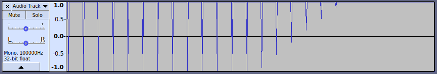
So here’s the full code:
(setf bias (snd-avg *track* 20 20 op-average))
(osc-pulse 5000 bias)
and here’s the result:
but let’s zoom in a bit at around the 4.0 second mark:
Observations:
If you zoom in on the PWM waveform near the start of the track, you will see that the pulse wave is not always complete.
This is because the width of the pulse is approaching zero, but we only have samples every 1/100000th second.
At the high frequency end of the “chirp”, the PWM signal only has about 5 pulses to define the waveform, so we can see that a 1000 Hz signal is approaching the limit of what a 5000 Hz pulse can handle.
Decoding:
If you try playing the PWM signal (turn the volume down a bit, it will be very loud), you will notice that it does not sound much like our original “chirp”. To recover our chirp sound, we need to decode the PWM signal. This is very easy to do. Just apply a low pass filter to remove the 5000 Hz carrier, and the result will be the “averaged” value of the pulses:
(lowpass8 *track* 1500)
LOWPASS8 is a steep lowpass filter.
The filter frequency of 1500 Hz is chosen to be far enough above our maximum signal frequency (1000 Hz) to not attenuate the signal too much, but well below our 5 kHz modulation frequency.
Note that at the low frequency end of the chirp, the demodulated output has distinct steps. This is because the 5000 Hz pulse wave has only 20 samples per cycle, so only 20 possible sizes for rectangular pulses, and because the change from one size rectangle to the next is so slow, our simple demodulator is unable to smooth out the steps.
Overall we can see that with a 100 kHz sample rate, and a 5 kHz pulse, our available audio bandwidth is around 200 Hz to 1000 Hz.