Let’s say I create a tone in Audacity float 32/384 environment, e.g. 5 seconds of 1kHz sine 0.8xFS.
I plot the spectrum with Hanning window, size 65536, and it will have a dynamic range of -144dB up to 1kHz, and -180dB above a few 1kHz.
I also save this tone as a pcm 16/44 in wav format.
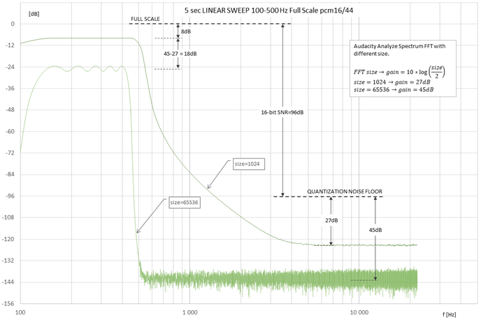
After this I open the file and the spectrum with Hanning window, size 65536, and it will have a dynamic range of -180dB with spikes to -120dB att 100, 200, 300…Hz in the whole band to 22kHz.
We should expect to see the noise floor due to quantization at -192dB for the pcm32/384 and at -96dB for the pcm16/44.
I’ve been using Audacity for some time so I have seen this “phenomena”, and I think it’s related to the FFT methodology.
Should I add 10log(size/2) [dB] to the FFT magnitude to represent the real noise floor?
Or what do I not understand?
That isn’t showing dynamic range of the audio, it’s just showing the limitations of FFT analysis. If the analysis (and graph) were “perfect”, there would be an extremely thin vertical line at 1000 Hz and the digital noise level would be way off screen at around -700 dB.
That isn’t showing dynamic range of the audio, it’s just showing the limitations of FFT analysis. If the analysis (and graph) were “perfect”, there would be an extremely thin vertical line at 1000 Hz and the digital noise level would be way off screen at around -700 dB.
Yes, I know.
But the sound is not perfect, so the two pcm tracks I created (32/384 and 16/44) contain a quantization noise level which should be expected at -192 and -96dB.
That’s why I suggested to add 10log(size/2) to account for the FFT process itself. I.e to add 10log(65536/2)=45dB to the exported magnitude.
The quantize noise floor for 32-bit float is below -700 dB. Audacity doesn’t support 32-bit integer, but yes that would have a quantize noise level of around -190 dB.
I’m not clear what precisely you mean by “this phenomena”.
I’m not clear what precisely you mean by “this phenomena”.
The FFT process itself uses some processing gain resulting in a lower magnitude than it actually is. The higher “size” in the FFT, the higher processing gain. You see it by analyzing any tone and looking at the magnitude with different “size” in FFT. It’s very obvious if you analyze a sweep.
So, if the noise in a digitized file is random (like quantization noise), the FFT process will lower the noise floor by 10log(size/2).
Therefore, if I want to estimate the dynamic range of a digitized file from FFT Analyze Spectrum, I have to raise the noise floor shown by FFT by 10log(size/2).
It’s not an error, it’s a phenomenon, similar to narrowing bandwidth with an analog spectrum analyzer.
The apparently higher noise level at low frequencies is misleading. If you plot a higher frequency sine tone (say 10 kHz) and set the X scale to linear, you will see that the noise floor is fairly evenly distributed.
The quantize error for 16-bit data is +/- 0.5/(2^15) = 1/65536 = 0.000015259
Converted to dB:
20 * log 0.000015259 = -96.3 dB
However, this error is distributed randomly across 32768 frequency bins, so we see random values well below -96 dB.
Note that for 32-bit float, the error is not determined by the smallest 32-bit value, but by the fact that Audacity exports the values rounded to 6 decimal places (-120 dB).
this error is distributed randomly across 32768 frequency bins, so we see random values well below -96 dB.
Yes, and the core of my question is how big this “well below” value is, because it should be compensated for when looking at FFT:s for digitized/converted files.
I think the value is 10*log(size/2), and I wonder if someone can confirm that.
The apparently higher noise level at low frequencies is misleading. If you plot a higher frequency sine tone (say 10 kHz) and set the X scale to linear, you will see that the noise floor is fairly evenly distributed.
Yes, it doesn’t need to be high frequencies. A low freq sine sweep show the “ski hill” better for low size FFT. But my question is still the same, and I try to illustrate it here (avoiding misleading parts):
Actually, I also wonder why the frequencies below the tone gets a higher noise level for low size FFT:s.
And I also wonder how much the FFT lowers the tone peak magnitude. I thought it was -6dB for a 0dBFS tone, but it seems it depends both on the bit depth and the FFT size.
For natural sound, it’s random. It’s “possible” (but highly unlikely) that one FFT bin could be entirely empty, which would represent -infinity dB for that bin.
What we do know is that the range for the error in any sample value is +/- 0.5/32768
Where we might see a zero value is in the DC component, if the waveform is symmetric around zero. However, Audacity’s Plot Spectrum omits the DC component.
For a sine tone, it would be possible to calculate the actual error for each sample value by calculating the exact theoretic sample value:
Amplitude*sin((omega * time) + phase)
and subtract that from the closest 16-bit value.
When converting from 32-bit float to an integer format, it is usual to apply “dither”, which shapes the distribution of the noise floor so that more of it lies in the very high frequency range where human hearing is less sensitive to low level noise. Audacity applies “shaped dither” by default, though other options are available (Quality Preferences - Audacity Manual)
What we do know is that the range for the error in any sample value is +/- 0.5/32768
Yes, and this is valid for the size=65536. For arbitrary size it is +/-0.52/size.
And it means the range for random noise (which is the case for quantization noise) then is 10log(size/2).
Thanks!
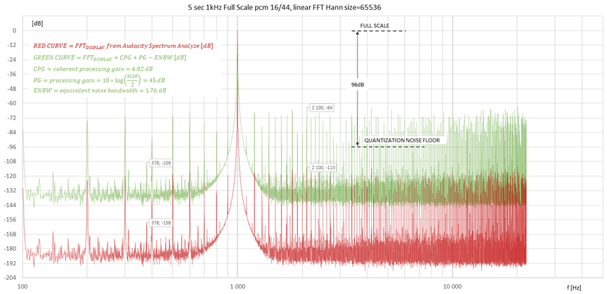
It should also be possible to estimate how much gain the FFT process use from the signal itself, not just the noise, i.e. CPG (coherent power gain) and SL (scalloping loss). When using Hanning window, I think CPG=6dB and maximum SL=1.5dB.
The energy on each side of the signal (e.g. the ski hill) is due to leakage (smearing) in the FFT process. It can be measured by combining the highest sidelobe in dB and the fall off in dB/octave. For a Hanning window, the highest sidelobe is -32dB and the fall off is -18dB/oct.
I still don’t know why the noise floor for frequencies below the signal is much higher than the noise floor above the signal. E.g. -144dB below compared to -180dB above the 1kHz signal in the first image in this thread.
It would be nice to be able to calculate (estimate) the true magnitude in the frequency range for both noise and broadband signals based on the FFT spectrum created in Audacity. I think it’s only a matter of calculating the CPG and the ENBW (equivalent noise bandwidth).
No, this is valid for 16-bit samples.
For 8-bit samples, each sample value is an exact multiple of 1/(2^8), and 24-bit samples have values that are exact multiples of 1/(2^24)
It isn’t. As I suggested previously, try using linear scale for the X (frequency) axis.
The values returned from Plot Spectrum are normalized such that a 0 dB (peak) sine wave is measured as 0 dB.
I’m getting the impression that you are trying to deduce something that doesn’t exist by comparing discrete frequencies to broadband noise. For noise, you can’t say that the level is …dB at …Hz, because we don’t / can’t know if there is any sound at “exactly” that frequency - all we can do is to measure how much is within each specified “frequency range”, and those are the figures that we see in the spectrum data.
No, this is valid for 16-bit samples.
For 8-bit samples, each sample value is an exact multiple of 1/(2^8), and 24-bit samples have values that are exact multiples of 1/(2^24)
It is very obvious that the noise floor change when the FFT size change, even if the bit depth of the file is the same.
But of course the bit depth of the file also change the noise floor.
It isn’t. As I suggested previously, try using linear scale for the X (frequency) axis.
Great. Of course, I forgot that. Sorry.
I tried this and it looks much better with linear scale in case I use high size. Like in image below. Thanks.
I’m getting the impression that you are trying to deduce something that doesn’t exist by comparing discrete frequencies to broadband noise. For noise, you can’t say that the level is …dB at …Hz, because we don’t / can’t know if there is any sound at “exactly” that frequency - all we can do is to measure how much is within each specified “frequency range”, and those are the figures that we see in the spectrum data.
I’m just trying to add an estimation of the gain/loss used by the FFT process itself, because this gain/loss is not in the sound. It is just a consequence of the FFT process.
That’s like saying that two countries are further apart when measured in kilometers rather than miles.
Hehe, yes it is. But it doesn’t have to be.
It would be really good if what’s shown in the FFT could be correlated to what is actually in a sound file.
Audacity could be used for many types of measurements.
Good looking graphs by the way. How are you doing those?
Thanks. The export from Audacity is just pasted to MS Excel.
I think this article describes the relevant issues quite clearly (and without getting too heavily into the mathematics): > https://www.ap.com/blog/fft-spectrum-an > … t-scaling/
Thanks.
The article confirms that the true noise floor can be estimated by adding 10*log(size/2) to the noise floor calculated in the FFT.